What Is a PCA? A Comprehensive Guide

Principal Component Analysis (PCA) is a powerful technique used to simplify complex data. Are you looking for a way to reduce the dimensions of your data while retaining its essence? This comprehensive guide on WHAT.EDU.VN will explore what PCA is, how it works, and why it’s an invaluable tool. Learn about dimensionality reduction, data analysis, and feature extraction.

1. Understanding Principal Component Analysis (PCA)

Principal Component Analysis (PCA) is a dimensionality reduction technique widely used in machine learning and data analysis. But what exactly is it? At its core, PCA is a method that transforms a large set of variables into a smaller one, called principal components, that still contains most of the information in the original dataset. This is achieved by identifying the directions, or components, in which the data varies the most.

Think of it this way: imagine you have a dataset with information about different types of fruits, including their color, size, weight, and sweetness. Each of these characteristics represents a variable. PCA helps you combine these variables into new, uncorrelated variables (principal components) that capture the most important differences between the fruits. For instance, the first principal component might represent a combination of size and weight, while the second might represent sweetness.

PCA is particularly useful when dealing with high-dimensional data, where the number of variables is large. Reducing the number of variables simplifies the data, making it easier to explore, visualize, and analyze. It also helps to reduce noise and improve the performance of machine learning models.

2. The Importance of Dimensionality Reduction

Why is dimensionality reduction so important? In many real-world scenarios, datasets can contain hundreds or even thousands of variables. Analyzing such datasets can be computationally expensive and time-consuming. Moreover, high-dimensional data can lead to overfitting in machine learning models, where the model learns the training data too well and performs poorly on new data.

Dimensionality reduction techniques like PCA address these challenges by reducing the number of variables while preserving the essential information. This leads to several benefits:

Simplified Data: Easier to understand and visualize.
Reduced Computational Cost: Faster analysis and model training.
Improved Model Performance: Less overfitting and better generalization.
Noise Reduction: Filtering out irrelevant or redundant information.

3. The Mathematics Behind PCA: A Simplified Explanation

While the underlying mathematics of PCA can seem daunting, the core concepts are relatively straightforward. Here’s a simplified explanation:

Standardization: The first step is to standardize the data, ensuring that each variable has a mean of 0 and a standard deviation of 1. This prevents variables with larger ranges from dominating the analysis.
Covariance Matrix: Next, the covariance matrix is calculated. This matrix shows how the variables in the dataset vary together. A positive covariance indicates that two variables tend to increase or decrease together, while a negative covariance indicates that they tend to move in opposite directions.
Eigenvectors and Eigenvalues: The eigenvectors and eigenvalues of the covariance matrix are then computed. Eigenvectors represent the directions of the principal components, while eigenvalues represent the amount of variance explained by each component. The eigenvector with the highest eigenvalue corresponds to the first principal component, which captures the most variance in the data.
Feature Vector: The eigenvectors are sorted by their eigenvalues in descending order, and a feature vector is created by selecting the top k eigenvectors, where k is the desired number of principal components.
Data Transformation: Finally, the original data is transformed into the new space defined by the principal components by multiplying the transpose of the original data by the transpose of the feature vector.

4. Step-by-Step Guide to Performing PCA

Let’s break down the process of performing PCA into a series of steps:

4.1. Data Preparation

The first step is to prepare your data for PCA. This involves cleaning the data, handling missing values, and ensuring that the data is in a suitable format.

Data Cleaning: Remove any irrelevant or inconsistent data points.
Missing Values: Impute or remove missing values.
Data Formatting: Ensure that the data is in a numerical format.

4.2. Standardization

As mentioned earlier, standardization is a crucial step in PCA. It ensures that each variable contributes equally to the analysis, preventing variables with larger ranges from dominating the results. To standardize the data, subtract the mean and divide by the standard deviation for each value of each variable.

4.3. Covariance Matrix Calculation

The covariance matrix shows how the variables in the dataset vary together. It is a symmetric matrix where each element represents the covariance between two variables. The covariance between two variables x and y is calculated as:

Cov(x, y) = Σ [ (xᵢ – μₓ) (yᵢ – μᵧ) ] / (n – 1)

where:

xᵢ and yᵢ are the individual values of the variables x and y
μₓ and μᵧ are the means of the variables x and y
n is the number of data points

4.4. Eigenvalue Decomposition

Eigenvalue decomposition is a mathematical technique used to find the eigenvectors and eigenvalues of a matrix. In the context of PCA, we perform eigenvalue decomposition on the covariance matrix to find the principal components.

Eigenvectors: Represent the directions of the principal components.
Eigenvalues: Represent the amount of variance explained by each component.

4.5. Feature Vector Creation

The feature vector is a matrix that contains the eigenvectors of the principal components that we want to keep. To create the feature vector, sort the eigenvectors by their eigenvalues in descending order and select the top k eigenvectors, where k is the desired number of principal components.

Principal Component Analysis Example:

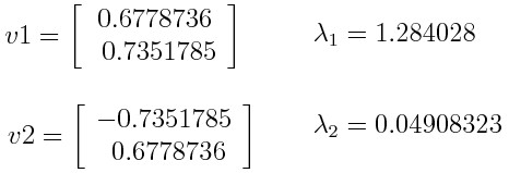
Let’s say we have a dataset with two variables, x and y, and we have calculated the eigenvectors and eigenvalues of the covariance matrix as follows:

Principal Component Analysis Example

If we rank the eigenvalues in descending order, we get λ1 > λ2, which means that the eigenvector that corresponds to the first principal component (PC1) is v1 and the one that corresponds to the second principal component (PC2) is v2.

If we want to reduce the dimensionality of the data to one dimension, we can discard the eigenvector v2 and form a feature vector with v1 only:

4.6. Data Transformation

Finally, the original data is transformed into the new space defined by the principal components by multiplying the transpose of the original data by the transpose of the feature vector. This results in a new dataset with a reduced number of variables that still captures most of the information in the original dataset.

5. Practical Applications of PCA

PCA has a wide range of applications in various fields. Here are some examples:

Image Compression: PCA can be used to reduce the size of images while preserving their essential features.
Facial Recognition: PCA can be used to extract the most important features from facial images, which can then be used for recognition.
Bioinformatics: PCA can be used to analyze gene expression data and identify patterns that are associated with different diseases.
Finance: PCA can be used to reduce the number of variables in financial models, making them easier to analyze and interpret.
Data Visualization: PCA can be used to reduce the dimensionality of data to two or three dimensions, allowing it to be visualized in a scatter plot.

6. Advantages and Disadvantages of PCA

Like any technique, PCA has its advantages and disadvantages.

Advantages:

Dimensionality Reduction: Reduces the number of variables in a dataset, simplifying the data and making it easier to analyze.
Noise Reduction: Filters out irrelevant or redundant information, improving the quality of the data.
Improved Model Performance: Reduces overfitting and improves the generalization of machine learning models.
Data Visualization: Allows high-dimensional data to be visualized in two or three dimensions.

Disadvantages:

Information Loss: Reducing the number of variables inevitably leads to some information loss.
Interpretability: The principal components are often difficult to interpret, as they are linear combinations of the original variables.
Standardization Requirement: PCA requires the data to be standardized, which can be a time-consuming process.
Linearity Assumption: PCA assumes that the relationships between the variables are linear, which may not always be the case.

7. PCA vs. Other Dimensionality Reduction Techniques

PCA is not the only dimensionality reduction technique available. Other popular techniques include:

Linear Discriminant Analysis (LDA): LDA is a supervised dimensionality reduction technique that aims to find the best linear combination of features that separates different classes.
t-Distributed Stochastic Neighbor Embedding (t-SNE): t-SNE is a non-linear dimensionality reduction technique that is particularly well-suited for visualizing high-dimensional data in two or three dimensions.
Autoencoders: Autoencoders are neural networks that can be trained to reduce the dimensionality of data.

The choice of which technique to use depends on the specific problem and the characteristics of the data. PCA is a good choice when the relationships between the variables are linear and the goal is to reduce the number of variables while preserving the most important information. LDA is a good choice when the goal is to separate different classes. t-SNE is a good choice when the goal is to visualize high-dimensional data in two or three dimensions. Autoencoders are a good choice when the relationships between the variables are non-linear.

8. Optimizing PCA for SEO

To optimize this article for SEO, we can use several strategies:

Keyword Research: Identify relevant keywords that people are searching for when looking for information about PCA.
Title Optimization: Use a clear and concise title that includes the main keyword.
Meta Description Optimization: Write a compelling meta description that summarizes the content of the article and encourages people to click through.
Header Optimization: Use descriptive headers that include relevant keywords.
Content Optimization: Write high-quality, informative content that is easy to read and understand.
Image Optimization: Use descriptive alt text for images that includes relevant keywords.
Internal Linking: Link to other relevant articles on your website.
External Linking: Link to high-quality external resources.

9. Frequently Asked Questions About PCA

Here are some frequently asked questions about PCA:

Question	Answer
What does a PCA plot tell you?	A PCA plot shows similarities between groups of samples in a data set. Each point on a PCA plot represents a correlation between an initial variable and the first and second principal components.
Why is PCA used in machine learning?	PCA reduces the number of variables or features in a data set while still preserving the most important information like major trends or patterns. This reduction can decrease the time needed to train a machine learning model and helps avoid overfitting in a model.
Is PCA a supervised or unsupervised learning technique?	PCA is an unsupervised learning technique, as it does not require labeled data. It identifies patterns and relationships in the data without any prior knowledge of the classes or categories.
How do I choose the number of principal components?	There are several methods for choosing the number of principal components, such as the elbow method, the scree plot, and the cumulative variance explained. The elbow method involves plotting the variance explained by each component and selecting the number of components at the “elbow” of the curve. The scree plot involves plotting the eigenvalues of each component and selecting the number of components before the eigenvalues start to level off. The cumulative variance explained involves selecting the number of components that explain a certain percentage of the total variance in the data.
What are the limitations of PCA?	PCA assumes that the relationships between the variables are linear, which may not always be the case. It also requires the data to be standardized, which can be a time-consuming process. Additionally, the principal components are often difficult to interpret, as they are linear combinations of the original variables.
Can PCA be used for non-linear data?	While PCA is a linear technique, it can be used for non-linear data by applying kernel PCA. Kernel PCA uses kernel functions to map the data into a higher-dimensional space where the relationships between the variables are more linear.

10. Conclusion: Unlock the Power of PCA with WHAT.EDU.VN

Principal Component Analysis is a powerful tool for dimensionality reduction and data analysis. By understanding the principles behind PCA and following the steps outlined in this guide, you can effectively simplify complex data, improve the performance of machine learning models, and gain valuable insights into your data.

Do you have more questions about PCA or other data analysis techniques? Visit WHAT.EDU.VN today and ask our experts for free guidance! We’re here to help you unlock the power of data.

If you’re facing challenges in finding quick and free answers to your questions, or if you’re unsure where to seek knowledgeable advice, WHAT.EDU.VN is your solution. We provide a free platform to ask any question and receive prompt, accurate responses. Our goal is to connect you with a community of experts who can share their knowledge and insights, making learning easy and accessible.

Ready to get your questions answered? Visit WHAT.EDU.VN and ask away!

Contact Us:

Address: 888 Question City Plaza, Seattle, WA 98101, United States
WhatsApp: +1 (206) 555-7890
Website: what.edu.vn